Statistics 101
Z-Test
Z-tests are statistical calculations that can be used to compare population means to a sample’s. The z-score tells you how far, in standard deviations, a data point is from the mean or average of a data set. A z-test compares a sample to a defined population and is typically used for dealing with problems relating to large samples (consider $n \geq 30$ as large enough to apply Central Limit Theorem for Means for any population). Z-tests can also be helpful when we want to test a hypothesis. Generally, they are most useful when the standard deviation is known.

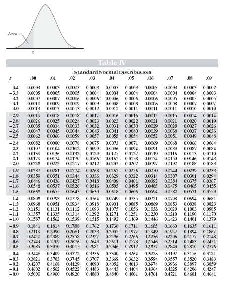
Z table; Source
The t-test can be categorized into two:
We are going to discuss each of cases in detail.
(1). One-Sample:
The one-sample z-test is used to test whether the mean of a population is greater than, less than, or not equal to a specific value. Because the standard normal distribution is used to calculate critical values for the test, this test is often called the one-sample z-test. The z-test assumes that the population standard deviation is known.
The workflow of the Test is as below:
Null Hypothesis ($H_0$): states that the population mean is equal to some value ($\mu_0$)
Alternative Hypothesis ($H_a$): states that the mean does not equal/is greater than/is less than $\mu_0$
Z-statistic: standardizes the difference between $\bar{x}$ and $\mu_0$
$ z = \frac{\bar{x} - \mu_0}{ s } = \frac{\bar{x} - \mu_0}{\frac{\sigma}{\sqrt{n}}} $
Formula for continuous data
Read the z-score table the p-value, probability that the sample mean was obtained by chance given $\mu_0$ is the popluation mean, using the calculated z-statistic.
- $H_0: \mu \leq \mu_0 \\ H_a: \mu > \mu_0 $
- $\rightarrow\ \\ \text{one-tail test on right-tail; p = area right of z}$
- $H_0: \mu \geq \mu_0 \\ H_a: \mu < \mu_0 $
- $\rightarrow\ \text{one-tail test on left-tail; p = area left of z}$
- $H_0: \mu = \mu_0 \\ H_a: \mu \neq \mu_0 $
- $\rightarrow\ \text{two-tail test; p = 2 * area past z}$
If the p-value is less than the predetermined value for significance, called $\alpha$ and is usually 0.05, reject the null hypothsis and accept the alternative hypothesis.
Example:
In 2015, millennials were watching 26.5 hours of TV a week with a standard deviation of 10 hours. Today, someone surveyed 50 millennials and found that they watch 24 hours of TV per week. Has the number of hours decreased?
Hypothesis:
$H_0: \mu \geq 26.5$
$H_a: \mu < 26.5$
$\bar{x}=24$
$n=50$
$s=\frac{\sigma}{\sqrt{n}}=\frac{10}{\sqrt{50}}=1.41$
The z-statistics is:
$z = \frac{\bar{x} - \mu_0}{ s } = \frac{\bar{x} - \mu_0}{\frac{\sigma}{\sqrt{n}}} = \frac{24-26.5}{1.41} = -1.77$
By looking at the z-score table above, $p(z \leq -1.77) \approx 0.0384$, p-value is less than 0.05 threshold, so, we can reject $H_0$ and coclude that the the number of hours has been decreased with 95% of confidence.
(2). Two-Sample:
The paired z-test may be used to test whether the mean difference of two populations is greater than, less than, or not equal to 0. Because the standard normal distribution is used to calculate critical values for the test, this test is often called the paired z-test. The paired z-test assumes that the population standard deviations ($\sigma$) are known.
Assume the two population are independent.
| $H_0: \text{means of the two population are equal}$ | $H_a: \text{means of the two population are unequal or one is greater than the other}$ | Test |
|---|---|---|
| $\mu_1 = \mu_2$ | $\mu_1 \neq \mu_2$ | Two-tail test |
| $\mu_1 \leq \mu_2$ | $\mu_1 > \mu_2$ | One-tail test: right-tail |
| $\mu_1 \geq \mu_2$ | $\mu_1 < \mu_2$ | One-tail test: left-tail |
z-statistic:
$ z = \frac{\bar{x_1}-\bar{x_2}}{\sqrt{\frac{S_1^2}{n_1} + \frac{S_2^2}{n_2} }} $
Formula for continuous data
Read the table of z-table for the p-value.
Example:
A Heart Study of Systolic Blood Pressure for men and women are shown as the table below. Suppose we now wish to assess whether there is a statistically significant difference in mean systolic blood pressures between men and women using a 5% level of significance.
| Men | Women |
|---|---|
| $n_1=1623$ $\bar{x_1}=128.2$ $s_1=17.5$ |
$n_2=1911$ $\bar{x_2}=126.5$ $s_2=20.1$ |
Hypothesis:
$H_0: \mu_1 = \mu_2$
(The means of two population are equal)
$H_a: \mu_1 \neq \mu_2$
(Because we want to see if two groups are different)
The z-statistics is:
$z = \frac{\bar{x_1}-\bar{x_2}}{\sqrt{\frac{S_1^2}{n_1} + \frac{S_2^2}{n_2} }} = \frac{128.2-126.5}{\sqrt{\frac{17.5^2}{1623} + \frac{20.1^2}{1911} }} \approx 2.688$
By looking at the z-score table above, $p(z \leq -2.688) \approx 0.0038$. The p-value, $2 \times p(z \leq -2.688) \approx 0.0076$, less than 0.05 threshold, so, we can reject $H_0$ and coclude that there is no statistically significant difference in mean systolic blood pressures between men and women.
