
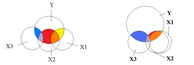
Multicollinearity Example; Source
In statistics, multicollinearity (also collinearity) is a phenomenon in which one predictor variable in a multiple regression model can be linearly predicted from the others with a substantial degree of accuracy. – Wiki
When independent variables in the regression model are highly correlated to each other, the multicollinearity usually happens. And, it could be hard to interpret models and it may face overfitting problem.
For example, a monthly sales record for this year might be choosen to build a regression model. However, the way we choose to monthly sales record as independent variables could lead the wrong conclusion. Let’s say we have quartly sales record for 2020 and monthly sales records 2020 as our independent variables. And we will see that these features are highly correlated with each other. Because Q1 sales record consist of Jan, Feb and March records and vice versa.
What is the problem of Multi-Collinearity?
When independent variables are highly correlated, any change of a variable will cause a chain rule effect on one variable to another variable. The model, then, will have misleading results for incorrect conclusion.
- It would be hard to identify significant variables for the model
- Coefficient Estimates would not be stable and it would be hard to interpret the model
- The unstable nature of the model may cause overfitting. When out of sample data applies, the accuracy will drop significantly
PS: Depending on the situation, it may not be a problem if a model has slightly or moderately collinearity issue. However, it is strongly advised to solve the issue if severe collinearity issue exists (e.g. Correlation > 0.8 between 2 variables or Variance inflation factor(VIF) > 20 )
There are many methods to check if Multi-Collinearity occurs. The simple methods are:
- Correlation Matrix
- Variance Inglation Factor (VIF)
(1). Correlation Matrix:
Here, we use the toy dataset, boston house prices dataset, from sklearn as the example.
from sklearn.datasets import load_boston
boston_dataset = load_boston()
print(boston_dataset.keys())
dict_keys(['data', 'target', 'feature_names', 'DESCR', 'filename'])
Use DESCR method can get the document of the dataset.
print(boston_dataset.DESCR).. _boston_dataset:
Boston house prices dataset
---------------------------
**Data Set Characteristics:**
:Number of Instances: 506
:Number of Attributes: 13 numeric/categorical predictive. Median Value (attribute 14) is usually the target.
:Attribute Information (in order):
- CRIM per capita crime rate by town
- ZN proportion of residential land zoned for lots over 25,000 sq.ft.
- INDUS proportion of non-retail business acres per town
- CHAS Charles River dummy variable (= 1 if tract bounds river; 0 otherwise)
- NOX nitric oxides concentration (parts per 10 million)
- RM average number of rooms per dwelling
- AGE proportion of owner-occupied units built prior to 1940
- DIS weighted distances to five Boston employment centres
- RAD index of accessibility to radial highways
- TAX full-value property-tax rate per $10,000
- PTRATIO pupil-teacher ratio by town
- B 1000(Bk - 0.63)^2 where Bk is the proportion of blacks by town
- LSTAT % lower status of the population
- MEDV Median value of owner-occupied homes in $1000's
:Missing Attribute Values: None
:Creator: Harrison, D. and Rubinfeld, D.L.
This is a copy of UCI ML housing dataset.
https://archive.ics.uci.edu/ml/machine-learning-databases/housing/
This dataset was taken from the StatLib library which is maintained at Carnegie Mellon University.
The Boston house-price data of Harrison, D. and Rubinfeld, D.L. 'Hedonic
prices and the demand for clean air', J. Environ. Economics & Management,
vol.5, 81-102, 1978. Used in Belsley, Kuh & Welsch, 'Regression diagnostics
...', Wiley, 1980. N.B. Various transformations are used in the table on
pages 244-261 of the latter.
The Boston house-price data has been used in many machine learning papers that address regression
problems.
.. topic:: References
- Belsley, Kuh & Welsch, 'Regression diagnostics: Identifying Influential Data and Sources of Collinearity', Wiley, 1980. 244-261.
- Quinlan,R. (1993). Combining Instance-Based and Model-Based Learning. In Proceedings on the Tenth International Conference of Machine Learning, 236-243, University of Massachusetts, Amherst. Morgan Kaufmann.
Convert the toy dataset into pandas dataframe.
import pandas as pd
df = pd.DataFrame(boston_dataset.data, columns=boston_dataset.feature_names)
df.head()
Add the dependent variable, target variable, into dataframe.
df['MEDV'] = boston_dataset.target
df.head()
# plot color scaled correlation matrix
corr = df.corr().round(2)

# Draw the heatmap with the mask and correct aspect ratio
import seaborn as sns
import matplotlib.pyplot as plt
import numpy as np
plt.figure(figsize=(15,10))

## Generate a mask for the upper triangle
mask = np.zeros_like(corr, dtype=np.bool)
mask[np.triu_indices_from(mask)] = True

## Generate a custom diverging colormap
cmap = sns.diverging_palette(300, 210, as_cmap=True)

## annot = True to print the values inside the square
hm=sns.heatmap(data=corr, mask=mask, cmap=cmap, vmax=.3, center=0, annot=True,
            square=True, linewidths=.5, cbar_kws={"shrink": .5})
plt.title('Correlation Plot')
plt.show();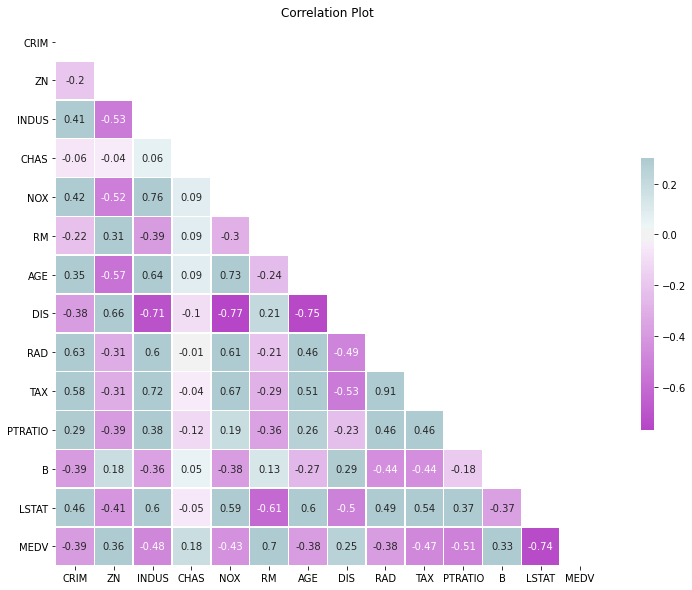
Heatmap helps select variables for a regression model by looking at the correlation matrix. The higher absolute values of correlation between the pairs of dependent variable and independent variable could be the good indicator for choosing the predictors of a regression model.
Usually, to identify the multicollinearity issue, we will check a pair of independent variables to see if its correlation exceeds 0.8. Here, the correlation matrix shows no strong sign of multicollinearity issue between idependent variables on this dataset.
(2). Variance Inglation Factor (VIF):
Use Variance Inflation Factor (VIF) for each independent variable. VIF determines the strength of the correlation between the independent variables. It is predicted by taking a variable and regressing it against every other variable.
VIF formula:
$ \text{VIF} = \frac{1}{1-R^2} $
$R^2$ value is determined to find out how well an independent variable is described by the other independent variables (a regression that does not involve the response variable Y). A high value of $R^2$ means that the variable is highly correlated with the other variables.
So, the closer the $R^2$ value to 1, the higher the value of VIF and the higher the multicollinearity with the particular independent variable.
# Compute VIF data for each independent variable
def calc_vif(X):
    """
    expect: X is a dataframe
    modify: calculate the VIF values
    return: return a dataframe
    """
    from statsmodels.stats.outliers_influence import variance_inflation_factor
    import pandas as pd
    # Calculating VIF
    vif = pd.DataFrame()
    vif["features"] = X.columns
    vif["VIF"] = [variance_inflation_factor(X.values, i) for i in range(X.shape[1])]

    return(vif)
Run the calc_vif function to get the VIF for each of independent variables.
X = df.iloc[:,:-1]
calc_vif(X)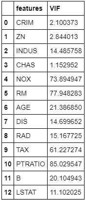
If VIF value is higher than 10, it is usually considered as having high correlation with other independent variables, meaning it can be predicted by other independent variables in the dataset.
PS: Although correlation matrix and scatter plots can also be used to find multicollinearity, their findings only show the bivariate relationship between the independent variables. VIF is preferred as it can show the correlation of a variable with a group of other variables.
How to fix Multi-Collinearity issue?
- Variable Selection
- Variable Transformation
- Principal Component Analysis
(1). Variable Selection:
Dropping one of the correlated features will help in bringing down the multicollinearity between correlated features.
X = df.drop(['NOX','RM','PTRATIO','TAX','MEDV'],axis=1)
calc_vif(X)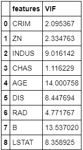
By removing the ‘NOX’,’RM’,’PTRATIO’,’TAX’ columns, the VIF has been reduced.
(2). Variable Transformation:
Transfromation can be done by combining two independents variables.
df2 = df.copy()
df2['INDUS_at_B_and_AGE'] = df.apply(lambda x: x['B'] - x['INDUS'] - x['AGE'],axis=1)
X = df2.drop(['INDUS','B','AGE', 'NOX','RM','PTRATIO','TAX','MEDV'],axis=1)
calc_vif(X)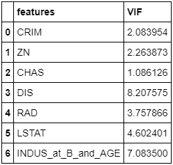
Here we can see the numbers are below 10 with variable transformation.
(3). Principal Component Analysis:
Principal Component Analysis (PCA) is commonly used to reduce the dimension of data by decomposing data into the number of independent factors. It has many applications like simplifying model calculation by reducing the number of predicting factors. Here, we use the character of variable independency for PCA to remove multi-collinearity issue in the model.
# Create the new data frame by transforming data using PCA
import numpy as np
from sklearn.decomposition import PCA
pca = PCA(n_components=7)
components=pca.fit_transform(X)
componentsDf=pd.DataFrame(data=components,columns=['component 1','component 2','component 3','component 4','component 5','component 6','component 7'])
print(componentsDf)
# Calculate VIF for each variable in the new data frame
X = componentsDf
calc_vif(X)
component 1 component 2 ... component 6 component 7
0 -53.445128 3.473428 ... -0.803652 -0.100734
1 -33.515130 -13.164395 ... 1.117063 -0.054929
2 -47.350198 -13.865980 ... 0.920758 -0.074221
3 -69.227443 -15.620510 ... 1.955364 -0.051563
4 -63.045406 -15.317811 ... 2.046793 -0.042474
.. ... ... ... ... ...
501 -33.545110 -13.279538 ... -1.389770 -0.117042
502 -30.888674 -13.011081 ... -1.590357 -0.123976
503 -16.782641 -11.514703 ... -1.771067 -0.138481
504 -15.013089 -11.431990 ... -1.518889 -0.129497
505 -26.854324 -12.550401 ... -1.397484 -0.122386
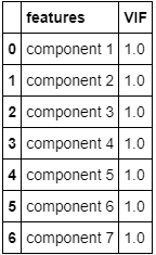
The PCA analysis seems to work very well on solving multi-collineartiy issue but model interpretation will be lost. And, when out of sample data is used to for predicting, the PCA transformation needs to be implemented again. Thus, we should try our best to reduce the correlation by selecting the right variables and transform them if needed.
Conclusion
Multicollinearity may not be a problem every time. The need to fix multicollinearity depends primarily on the below reasons:
- When you care more about how much each individual feature rather than a group of features affects the target variable, then removing multicollinearity may be a good option
- If multicollinearity is not present in the features you are interested in, then multicollinearity may not be a problem.
Reference:
Multicollinearity in Regression
What is Multicollinearity?